Membrane Cleaning Strategies: Extend Life and Reduce Downtime of Filtration Systems
Membrane Cleaning Strategies: Extend Life and Reduce Downtime of Filtration Systems
Membrane cleaning strategies for wastewater membranes that are vague or generic cost plants time and money; this guide gives operators and engineers practical, chemistry-specific tactics to cut unplanned downtime and extend membrane life. You will learn how to identify dominant foulants, set monitoring and CIP triggers with numeric thresholds, and run physical and chemical cleanings with proven concentrations, temperatures, and contact times matched to common membrane materials. The article also includes SOP templates, automation decision rules, and simple cost trade offs to help you justify pretreatment or CIP upgrades.
1. Identify Dominant Fouling Mechanisms in Wastewater Membranes
Start with the dominant foulant. Identifying whether the problem is primarily organic, particulate/colloidal, biological, or inorganic scaling is the single most practical action you can take to make cleaning effective and to avoid unnecessary chemical use. Treat cleaning as diagnosis-driven maintenance, not calendar-driven chemistry.
Onsite indicators that point to foulant type
- Organic fouling: rising
TMPwith higher UV254/TOC in feed and greasy or odorous deposits on module housings - Particulate or colloidal fouling: sudden turbidity spikes, higher particle counts, and poor backwash recovery after hydraulic cleaning
- Biofouling: gradual, persistent
TMPincrease, slimy deposits on autopsied fibers, high ATP readings and rapid re-growth after short disinfection - Inorganic scaling: patchy hard deposits, localized pressure steps, white or reddish crusts (calcium, silica, iron), and poor response to alkaline cleaners
Measurement choices matter. Use a mix of trend and spot tools: TMP and normalized flux for trends; turbidity and particle counters for solids; SDI/MBR-specific indices for feed quality; ATP or microscopy to confirm active biomass; and periodic chemical analysis for hardness, iron, and silica. The EPA membrane filtration guidance manual is a practical reference for setting up these tests.
Practical tradeoff: ATP gives rapid evidence of living biomass but does not measure extracellular polymeric substances that bind biofilm. Relying on ATP alone leads to false negatives for entrenched biofilm where enzymatic or oxidizing steps are required. Budget for one confirmatory lab test per unusual event.
Concrete example: A municipal UF train treating secondary effluent showed a steady TMP climb after a series of storm inflows. Online UV254 increased while particle counts stayed stable, pointing to soluble microbial products. Operators switched from routine backwashes to a targeted alkaline-enzymatic CIP sequence and restored permeability within two CIP cycles, avoiding premature membrane replacement.
Judgment you will not hear from sales reps: do not default to broad-spectrum oxidants at first sign of fouling. Oxidants can damage sensitive polymers and mask the true foulant by killing biomass without removing EPS or inorganic binders. A short diagnostic campaign – one or two focused tests plus a physical-cleaning recovery check – will give a higher return than immediately escalating chemical strength.
If a foulant diagnosis is unclear after basic onsite tests, pause and run one targeted analytical test (ATP, particle size distribution, or ion scan) before changing CIP chemistry.
2. Monitoring Metrics and Cleaning Triggers
Act on trends, not single blips. Set automated rules that combine a persistent decline in normalized permeability with a failed post-physical-clean recovery or a secondary signal (conductivity, UV254, turbidity) before launching a chemical CIP.
Core metrics and the decision logic
| Metric | What it flags | Practical trigger | Immediate action |
|---|---|---|---|
| Normalized flux (temperature/viscosity corrected) | Loss of hydraulic permeability from organics/colloids and early biofilm | 12–15% decline versus 7‑day rolling median sustained for 6–12 hours | Raise operator alert; run scheduled backwash; if post-backwash recovery <85% schedule CIP |
| Transmembrane pressure (TMP) gradient | Pressure build-up across modules, often particulate or cake layer | Increase of 0.15–0.4 bar not recovered by instantaneous backwash | Initiate additional physical cleaning (air scour/backpulse); if unrecovered, flag CIP |
| Permeate conductivity / salt passage (RO) | Early indicator of scaling or membrane damage | Permeate conductivity increase >10% above baseline for two consecutive readings | Pause high-flux operation, check antiscalant feed, then run targeted acid cleaning if confirmed |
| UV254 / online TOC | Rise in soluble organics that predict biofouling and EPS growth | 20% increase over baseline during a 24-hour window | Consider enzymatic/alkaline sequence and verify coagulation/pretreatment performance |
Normalize intelligently. Use a viscosity correction when comparing flux across temperature swings; a practical quick formula is Jn = J * (mu / mu_ref) where mu is feed viscosity. Run comparisons against a rolling 7-day median to avoid reacting to short disturbances from storms or process upsets.
Multi-parameter triggers reduce false alarms. Configure a two-of-three rule (normalized flux, TMP, plus one quality probe) with a 1–12 hour persistence window before auto-starting a CIP. Hard automation without confirmation wastes chemicals and shortens membrane life; soft alarms route to operator review first.
- Implement these steps in SCADA: define baselines (7-day median), add viscosity correction to flux, set persistence window, and require confirmation from a secondary sensor before enabling automated CIP.
- Validate weekly for 8 weeks: review false positives and adjust persistence or threshold to balance chemical use and downtime.
- Document every trigger event: store pre- and post-clean metrics for trend analysis and quarterly threshold tuning.
Concrete example: An industrial RO skid began to show a steady 13% drop in normalized flux over 10 hours while permeate conductivity crept up 12%. The plant used a two-parameter trigger, paused high-recovery operation, checked antiscalant dosing, and ran a short acid CIP. The cleaning restored design flux and avoided a costly emergency shutdown and membrane swap.
Trigger only when persistence and confirmation align: a short spike is an alarm, a sustained, multi-sensor trend is a cleaning trigger.
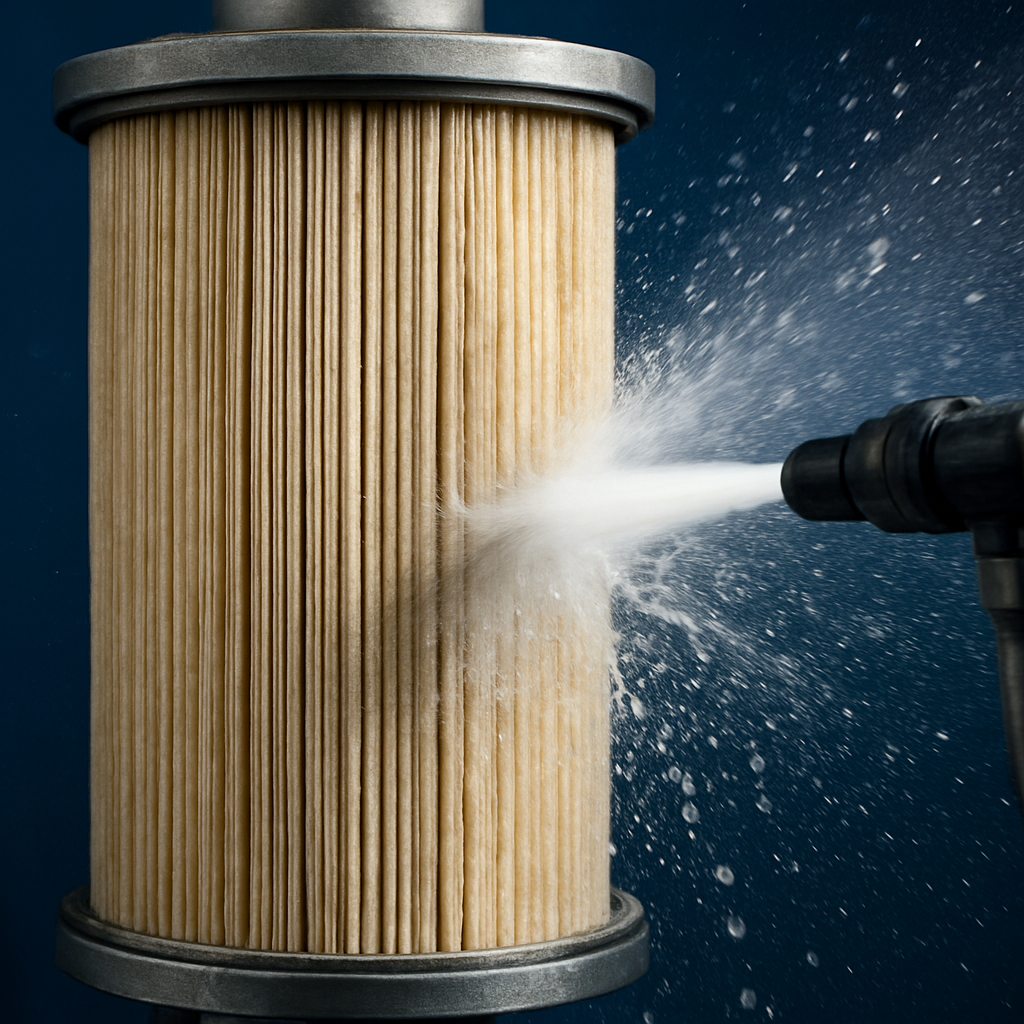
3. Physical Cleaning Techniques to Maximize Time Between CIP Operations
Physical cleaning is the cheapest, highest-frequency tool you have to delay chemical CIP. When done right, targeted hydraulic and pneumatic actions recover most reversible fouling, save chemicals, and smooth plant operations — but they require precise sequencing and acceptance of tradeoffs: more water use, higher pump cycling, and potential mechanical wear if abused.
Core physical methods and where they work
Backflush/backpulse: short, high-flow reversals dislodge cakes and trapped solids on UF/MF and hollow-fiber modules. Use permeate when feed quality would recontaminate fibers. Tradeoff: uses permeate or filtered water and fast valve action increases wear on piping and seals.
Air scour (hollow fiber): combine intermittent air bursts with low-pressure water flushes; air agitates biofilm and cake so hydraulic pulses remove it more effectively. Limitation: over-scouring abrades fibers — follow manufacturer air rates and cycle durations.
Forward flush and surface shear: for spiral-wound and RO, a high-velocity forward flush at controlled pressure can shear off soft deposits without reverse flow. Consideration: polyamide RO elements tolerate only limited pressure/oxidant exposure; check compatibility before aggressive hydraulic cleaning.
- Practical targets: set backpulse durations between 30 and 90 seconds and monitor flux recovery after each cycle; aim for clear, reproducible recovery signals rather than single-event spikes.
- Air/hydraulic sequencing: use alternating patterns (e.g., air burst then immediate short backflush) rather than continuous air to reduce abrasion and improve particulate removal.
- Tubular/plate systems: implement sponge-ball or pigging runs on return lines and clean-in-place circulation at moderate velocities to remove fouling layers inaccessible to simple backwash.
Operational trade-offs to weigh: increasing frequency or intensity of physical cleaning reduces chemical use but raises energy, water consumption, and mechanical wear. In practice, adjust physical cleaning until marginal benefit on flux recovery flattens — that is your economic sweet spot. Over-cleaning physically can shorten membrane life faster than modest, well-timed CIPs.
Concrete example: At a 50,000 PE municipal UF installation, operators redesigned the backwash sequence to include paired air-scour bursts and a forward flush using filtered permeate. Chemical CIP frequency fell by roughly 40 percent and unscheduled downtime dropped; however, the plant introduced a preventive check on fiber integrity and replaced air valves more frequently, an operational cost the team accepted because total lifecycle cost declined.
Common mistake operators make: believing any increase in hydraulic aggressiveness is better. In reality, indiscriminate high-pressure or continuous air-scour damages modules and produces marginal returns. Start conservative, measure post-clean flux reproducibility, then increase intensity in controlled steps.
Before changing physical-clean parameters, verify valve sequencing and air-supply conditioning, log cycle results for 90 days, and tie a simple decision rule in SCADA: if flux recovery after a physical cycle fails to meet your reproducible benchmark, escalate to a chemical CIP recipe. For design details and valve logic examples, see the plant automation guide and the EPA membrane manual at EPA Membrane Filtration Guidance Manual.
If a physical-clean sequence does not deliver consistent, repeatable flux recovery, escalate to a diagnostic (ATP, particle size, or microscopy) before increasing cleaning aggressiveness — the problem is often a change in foulant character, not insufficient hydraulics.
4. Chemical Cleaning Chemistries and Sequences
Chemistry is not a hammer; sequences win. Selecting a cleaning chemical by itself is a guess — choosing the right sequence to detach, solubilize, and flush the specific foulant is what restores flux without accelerating membrane wear.
- Alkaline cleaners (purpose and typical ranges): remove organic soils, grease and destabilize EPS. Practical working mixes are 0.1–0.5 wt percent NaOH often paired with 100–800 ppm oxidant when the membrane tolerates it; temperature 20–35 degrees C; contact 30–60 minutes under recirculation to maintain shear.
- Oxidants (purpose and cautions): sodium hypochlorite, peracetic acid, or hydrogen peroxide break biomass and denature proteins. Use them to accelerate EPS breakdown but only when the membrane polymer and seals tolerate oxidants — otherwise they cause irreversible damage and loss of selectivity.
- Acids and chelants (purpose): citric acid (0.5–2 wt percent) or low-strength HCl remove carbonate, iron and some siliceous scale; EDTA or phosphonate chelants (0.1–0.5 wt percent) complex metal ions and loosen hard deposits. Acid steps often follow alkaline/oxidant steps to remove the inorganic fraction that binds organics.
- Enzymatic cleaners (purpose and limits): proteases/amyloglucosidases target specific biofilm components and reduce mechanical scrubbing needs. Enzymes work best as part of an alkaline pretreatment; they require controlled temperature and are costly — good for recurring biofouling where oxidants are restricted.
- Neutral detergents and surfactants: useful as auxiliary additives to improve wetting and solubilization, but they complicate disposal and can increase foaming — use only when lab tests show a benefit.
Membrane material compatibility – practical limits
| Membrane polymer | Chemistry to avoid | Practical note |
|---|---|---|
| Polyamide (RO) | Free-chlorine oxidants and prolonged high-pH exposure | Use non-chlorine oxidants (H2O2, peracetic acid) with manufacturer approval; keep temperatures and pH within element limits and minimize contact time |
| PVDF / PES (UF/MF) | Strong acids at high temperature (avoid unnecessary extremes) | Generally tolerant of oxidants; verify seal and gasket materials for compatibility |
| Cellulose acetate | Strong alkali (prolonged high-pH exposure) | Acid-based cleaning preferred; alkali can hydrolyze polymer and reduce life |
Recommended sequence for mixed fouling and why it works. For combined organic/bio/inorganic layers, run an alkaline solubilization step first (alkali ± enzyme/low-dose oxidant) to soften organics and EPS, intermediate rinse, then an acid/chelant step to dissolve bound minerals. This order prevents organic matter from trapping precipitated salts during acid attack and reduces the likelihood of creating insoluble complexes that are harder to remove.
Tradeoffs and real constraints. Oxidants speed biofilm removal but can mask residual EPS and create a false sense of recovery if you only monitor ATP or kill-off indicators. Chelants pull metal ions into solution but increase dissolved metal load in waste streams and often require solids removal before discharge. Enzymes reduce mechanical force needs but increase OPEX and require inventory management.
Concrete example: An industrial facility treating metal-plating rinsewater was fighting iron-cemented deposits on UF modules. Operators ran a short EDTA soak (0.3 wt percent, 45 minutes, ambient temperature) to chelate iron, followed by a citric-acid rinse (1 wt percent, 30 minutes). Permeability recovered to within 90 percent of baseline after two cycles, avoiding membrane swap-out — but the plant added a solids-settling step to capture metal-rich precipitates before discharge.
Practical rule before scaling any recipe to a full train: bench or single-module trials with the same materials, temperature, and recirculation velocity you will use onsite. Small-scale validation reveals unintended reactions (precipitation, seal swelling, foaming) that are much cheaper to fix than a full-train CIP failure.
Disposal and safety you cannot skip. Neutralize acid/alkaline wastes to permit discharge limits, check residual oxidant with test strips before release, and expect chelants to keep metals in solution — which may violate local permits. See the EPA membrane filtration guidance manual for discharge handling and tie SOPs to your plant permit conditions.
Always validate a sequence on one module, log permeability and selectivity before and after, then scale to the remainder of the train once results are reproducible.
5. Step by Step CIP Template for UF/MF and RO Systems
Start with an executable script not a shopping list. The procedure below is a practical, test-then-scale CIP template you can run on one module or a single cassette, measure recovery, then move to full-train cleaning only when results are reproducible.
Operator checklist and sequencing
- Pre-checks: isolate the train, confirm bypass valves, verify all drains open, confirm chemical storage and PPE are ready, and log pre-clean
TMP, normalized flux, and permeate conductivity. - Pre-rinse: recirculate filtered permeate or clarified water until turbidity approximates normal permeate or drops to a low single-digit NTU band; sample at the module outlet to confirm solids removal before chemistry.
- Alkaline solubilization: raise solution to a high-alkaline pH target appropriate for your membrane polymer and seals; recirculate with moderate shear that equals at least one full volume turnover every 10 to 20 minutes; monitor pH and ORP and hold until flux improvement plateaus during the run.
- Intermediate rinse: flush until pH returns near feed baseline and conductivity stabilizes to avoid acid-alkali neutralization when you follow with an acid step.
- Acid / chelant step when scaling or metal fouling is suspected: apply an acidified or chelant-bearing solution with controlled recirculation; sample return line for dissolved metals and visible precipitation, and stop if solids exceed permitted handling thresholds.
- Final rinse and optional disinfectant: rinse until conductivity and pH match feed or permeate targets; if an antimicrobial soak is required, choose an oxidant compatible with the membrane and check residual oxidant before returning to service.
- Verification and hold: measure post-CIP normalized flux and salt passage or selectivity; do not reintroduce the train to full duty until permeability is within your acceptance band or a follow-up cycle is scheduled.
Practical control points to build into every run. Use pH and ORP as real-time controllers for chemistry strength rather than relying solely on weight percent dosing. Track a simple metric – percent flux recovery versus baseline – after each 20 to 30 minute interval during the CIP. Stop or adjust when incremental recovery falls below a small, pre-set threshold.
RO-specific adaptations. For polyamide RO, do not use free-chlorine steps. Instead, substitute non-chlorine oxidants or enzyme-assisted alkaline steps where vendor compatibility exists. Confirm permeate conductivity and salt passage immediately after cleaning to detect subtle membrane damage that flux alone will not show. If you use peroxide, plan an activated-carbon polish before discharge when required by permit.
Tradeoffs and a common operational mistake. Longer, gentler recirculation avoids seal stress and sudden osmotic shocks but consumes more operator time and solution volume. Operators often try one aggressive, high-strength CIP to save time – that tends to increase membrane polymer fatigue and unplanned element swaps. Stage intensity and validate on a module first.
Real-world use case: At a food processing plant using hollow-fiber UF, the team ran a single-cassette trial using an alkaline soak controlled by pH and ORP, followed by a citric-acid chelation pass. The cassette returned to near-design permeability within two runs and the plant avoided a midseason replacement. They recorded the exact pH and ORP profiles so the full-train CIP could be automated reliably.
Do not mix chemistries in the same recirculation batch and never rely on visual clarity alone to end a rinse – confirm pH, conductivity, and residual oxidant before returning a train to service.
Next consideration – convert the validated single-module recipe into a controlled automation sequence and tie start conditions to your monitoring triggers so CIP runs on signal, not on memory. For sequencing and alarm logic see the plant automation guidance in the plant automation guide and the operational limits in the EPA membrane manual.
6. Reducing Cleaning Frequency Through Pretreatment and Process Design
Core claim: investing in upstream pretreatment and deliberate process design reduces the need for frequent chemical CIP far more reliably than simply increasing cleaning intensity. Pretreatment lowers the foulant mass the membranes see, and process choices – not stronger chemistry – deliver the best ongoing reductions in downtime and lifecycle cost.
Pretreatment levers that cut fouling load
Target the dominant load, not everything. Use specific upstream fixes matched to the foulant: coagulation-flocculation plus clarification or fine-media filtration for colloidal and organic loads; dissolved air flotation (DAF) for fats, oils, and grease; cartridge or depth filters as polishing before RO; and antiscalant plus pH control for hardness-prone RO feeds. Small changes upstream often eliminate the need for a dozen aggressive CIPs downstream.
- Coagulation + media filtration: ferric or polyaluminum chloride ahead of a sand/dual-media filter to remove SMP and colloids that accelerate biofouling
- DAF or grease traps: remove FOG from food‑industry and high‑organic streams so UF backwashes remain effective
- Antiscalant and pH control for RO: dose and monitor based on LSI and silica risk rather than guessing on recovery targets
- Equalization and buffering: flatten turbidity and TOC spikes so membrane flux can run more consistently and physical cleaning recovers reliably
Process design choices that matter. Running membranes at lower specific flux, staging membrane trains (coarse then fine), scheduling periodic relaxation or short-duration offline windows for MBRs, and providing bypass for high-turbidity events all reduce cumulative fouling. These actions trade capacity or capex for fewer CIPs and longer element life – a deliberate economic choice, not a technical failure.
Practical screening rule. If a membrane train requires chemical CIP more than twice per month despite optimized physical cleaning, perform a pretreatment feasibility assessment before increasing chemical strength. In practice, pretreatment or modest flux reductions are frequently the cheaper, lower-risk solution than more aggressive chemistries.
Concrete example: A reclaimed-water facility treating industrial washwater added a DAF unit and upgraded to a 5 micron cartridge polish ahead of UF. Chemical CIP went from monthly to roughly once every 10 to 12 weeks, permeate quality stabilized, and unscheduled downtime fell. The plant accepted higher sludge handling and a 9-month payback on the pretreatment capex because membrane replacement deferrals and lower chemical OPEX were predictable.
Tradeoffs and limits you will face. Pretreatment requires footprint, operators, and produces additional solids or waste streams that must be managed. Reducing flux to avoid fouling increases membrane area needs and up-front cost. Anti-fouling coatings and surface modification can help but are not a substitute for removing foulant mass upstream; treat coatings as complementary, not primary.
Next consideration: run a one-month side-by-side trial with and without the proposed pretreatment and use CIP events, chemical use, and membrane permeability as your objective metrics before committing to full-scale installation.
7. Automation, Data, and Decision Support to Minimize Downtime
Direct claim: Automation and data do not eliminate cleaning needs — they shift failure modes from human error to configuration error. Well-implemented automation reduces unplanned outages by enforcing consistent CIP recipes, holding chemistry to setpoints, and preventing late-stage damage; poorly implemented automation runs chemicals on timers and accelerates membrane wear.
Core architecture for reliable automated CIP
Basic stack: a reliable sensor layer (pressure, flow, pH/ORP, conductivity, selectivity probe), a fast PLC for interlocks and valve sequencing, a recipe manager that stores tested CIP protocols, and a historian/analytics layer that enforces decision rules and retains event traces for audits. Integrate with SCADA alarms and a simple human-in-the-loop approval step for non-routine recipes.
- Automation-grade signals: valve position, pump speed, chemical dosing flow, and return-line turbidity so the system can detect incomplete recirculation or precipitation in real time.
- Decision inputs: a persistent multi-signal confirmation (e.g., sustained permeability loss plus failed physical-clean recovery and an elevated organics probe) before auto-starting a chemical CIP.
- Safety interlocks: lockouts for active maintenance, permit-based waste routing, residual oxidant checks before discharge, and a timeout that escalates to operator intervention if recovery stalls.
- Traceability: store full sensor and recipe logs for each CIP event so you can correlate long-term trends with recipe effectiveness and membrane aging.
Practical tradeoff: Automation buys consistency and repeatability but costs in configuration, testing, and governance. Expect a multi-week commissioning window to tune persistence windows, ORP/pH setpoints, and safe ramp rates. If you skip staged trials (single-module validation), automation magnifies mistakes across the whole train.
Judgment most operators miss: full automation without a decision-support layer is brittle. Add a simple rules engine that suggests, not forces, non-standard recipes and requires an operator sign-off for out-of-pattern events. This preserves the speed of automation while keeping diagnostics and human judgment in the loop.
Concrete example: A mid-size brewery with an ultrafiltration bank implemented PLC-driven CIP sequencing tied to live turbidity, ORP, and backwash recovery. The system auto-selected mild alkaline or an enzymatic recipe based on turbidity patterns and paused dosing if return-line solids were observed. Downtime for cleaning became scheduled and predictable, and the engineering team used the CIP logs to reduce unnecessary oxidant exposure after three months of tuning.
Implementation tips: start with conservative automation rules, require a one-module proof before scaling a recipe, and build dashboards that show recipe effectiveness over rolling windows. Connect to your permit compliance checks so automated discharge routing is never an afterthought — see the plant automation guide for control logic patterns and the EPA membrane manual for documentation best practices.
Automate what you have validated; validate what you plan to automate. Treat automation as a maintenance tool, not a replacement for diagnosis.
8. Cost, Downtime Trade Offs, and Lifecycle Impact
Straightforward point: lifecycle economics, not chemistry bravado, decide whether you tighten cleaning frequency, buy pretreatment, or automate CIP. Operating costs, downtime penalties, and membrane replacement timing interact; small changes in membrane life or unplanned outage hours produce outsized shifts in total cost per cubic meter.
Framework to evaluate choices: calculate a simple annualized cost per m3 that includes membrane amortization, chemical and consumable costs, labor for cleaning, added energy from elevated TMP, and a realistic dollar value for downtime (lost production, contractor mobilization, or penalty clause exposure). Run a sensitivity table that varies only two drivers at a time: membrane life and unplanned downtime hours. That shows which lever actually moves the needle on your site.
| Scenario | Annualized membrane cost (k$) | Other annual OPEX (chem, labor, energy, downtime) (k$) | Total annual cost (k$) | Cost per m3 ($/m3) |
|---|---|---|---|---|
| Aggressive CIP (monthly; higher chem/labor, longer life) | 35.7 | 110.0 | 145.7 | 0.020 |
| Reduced CIP (less chem; shorter element life, more downtime) | 62.5 | 115.0 | 177.5 | 0.024 |
Interpretation and tradeoff: the table is illustrative: aggressive CIP raises chemical and labor spend but can lower total annual cost if it meaningfully extends membrane life or prevents costly emergency outages. Conversely, cutting cleaning to save chemicals often shifts cost into higher amortization and unpredictable downtime. The result is site-specific; do not assume lower immediate OPEX equals lower lifecycle cost.
Concrete example: a mid-sized municipal plant treating ~20,000 m3/day compared two strategies. By adopting a targeted monthly CIP recipe plus improved pretreatment, the team pushed expected membrane replacement from 5 to about 7 years. Higher annual chemical and labor costs rose by ~40k$, but membrane amortization and unplanned outage costs fell enough that total annual cost per m3 dropped by roughly 15 percent. They funded the change by reallocating deferred capital for near-term replacements.
Automation and payback judgment: automation is not an automatic win. It pays when it reduces variability (fewer emergency cleanings and fewer human errors) and when labor or downtime costs are material. Use a conservative commission window: require 6–12 validated single-module runs before automating a recipe. If automation hardware and integration approach 0.5–1.0 million dollars, demand a two- to four-year payback using conservative downtime-avoidance numbers.
Final practical step: run a quick lifecycle-cost model on your plant with three scenarios (status quo, aggressive CIP + pretreatment, and reduced CIP). Tie the model to real outage logs and membrane replacement invoices. Use the results to set an explicit threshold for investments: if automation or pretreatment yields payback within your finance horizon at conservative downtime reductions, proceed; if not, optimize physical cleaning and diagnostics first.
9. Short Case Studies and Real Examples
Direct observation: short, focused case studies reveal what cleaning protocols actually survive plant realities. Laboratory recipes and vendor bulletins are necessary starting points but will not predict piping dead zones, unexpected precipitation, or regulatory limits on CIP wastes. Treat these studies as diagnostic templates, not final SOPs.
What the cases teach you in practice
Practical insight: a successful bench soak or single-module trial is necessary but not sufficient. Full-train scaling commonly fails because recirculation velocities, pump heat, or valve timing differ and create local precipitation or insufficient shear. Always measure return-line solids, ORP/pH transients, and flux recovery during scaling runs.
Field example: Orange County Water District runs multi-barrier pretreatment ahead of RO and pairs that with disciplined RO CIP windows and strict antiscalant control. The result is fewer emergency CIP runs and more predictable element life because the system reduces foulant mass sent to RO rather than relying solely on stronger chemistry at the RO stage. See a condensed profile of similar projects in our case studies page.
Manufacturer observation: Koch Membrane Systems documented municipal UF installations where optimizing coagulation plus air-scour timing reduced chemical CIP frequency by shifting removable load upstream and improving physical-clean effectiveness. The tradeoff was modest increases in valve and actuator maintenance, which the sites accounted for in lifecycle models.
Literature example: a Water Research paper on enzyme-assisted cleaning for MBRs showed meaningful reduction in entrenched biofilm when enzymes were sequenced with controlled alkaline steps and limited oxidant exposure on feed lines. Enzymes lowered mechanical scrubbing needs but introduced higher OPEX and more complex waste handling because breakdown products and chelated metals required different disposal routes.
- Common tradeoff across examples: stronger or more frequent chemical CIPs restore flux quickly but accelerate polymer fatigue and increase disposal complexity
- What consistently worked: invest first in pretreatment and precise physical-clean sequencing before escalating chemistry
- Operational control that matters: instrument the return line during full-train trials to catch precipitation or seal swelling early
Short trials that replicate full-train hydraulics catch 80 to 90 percent of scaling and precipitation issues before they reach the plant. Bench tests do not replace this step.
10. Implementation Checklist and Sample SOPs
Implementation fails without governance. A written checklist and a short, testable SOP reduce the two biggest failure modes: running a full-train CIP that was never validated, and letting operators improvise chemistry under pressure. Treat the checklist as an operational gate — nothing moves to full-train execution until the gate items are verified and signed off.
Minimum practical checklist (use before any full-train CIP)
| Checklist item | How to verify | Owner / When |
|---|---|---|
| Monitoring & alarm readiness | Confirm sensor calibration, historian traces available, and trigger rule simulated in SCADA | Instrumentation tech — before automation or scheduled CIP |
| Single-module validation | Run the exact recipe on one module; log flux/selectivity pre/post and inspect return line for precipitation | Operations engineer — 1–2 validation runs |
| Manufacturer compatibility confirmation | Written confirmation from membrane vendor or validated bench data on chemistry and max temperature | Process engineer — prior to first full-train run |
| Chemical inventory & waste plan | SDS on file, neutralization supplies staged, discharge route and permit acceptability confirmed | Environmental/ops — before dosing any chemical |
| PPE and safety briefing | Signed operator checklist and emergency contact list available at skid | Shift lead — start of shift |
| Automation dry-run | Simulate valve and pump sequencing without chemicals; confirm interlocks and alarms | Controls engineer — before automated CIP go-live |
| Post-CIP acceptance criteria defined | Document which metrics must return to acceptable band and who approves restart | Process engineer / plant manager — part of SOP |
Practical insight and tradeoff. A checklist enforces discipline but it is not a substitute for diagnostic thinking. Require operators to run a short diagnostic (single-module run or targeted probe check) when a CIP is triggered outside normal windows. This costs time up front but prevents misapplied chemistry that creates more downtime and speeds membrane aging.
Sample SOP skeleton (fields to complete and lock)
| SOP section | Required entries / example guidance |
|---|---|
| Purpose & scope | Define which trains/elements this SOP covers and the foulant scenario it addresses |
| Safety & permits | List PPE, spill response, and discharge permit conditions; include emergency neutralization steps |
| Pre-CIP checks | Isolation points, valve positions, sensor status, single-module validation reference, and chemistry batch ID |
| CIP sequence | Refer to the validated recipe file (exact concentrations, temperature limits set by vendor, recirculation flow/velocity target, and duration). Insert the single-module validation ID used to scale the recipe |
| Monitoring during CIP | Log pH/ORP, return turbidity, and temperature at set intervals; stop criteria and escalation steps if solids appear |
| Post-CIP verification | List required checks (flux, conductivity or selectivity probe, visual inspection) and the authority to return the train to service |
| Documentation & change control | Where to store run logs, how to submit a recipe change request, and training signoffs required for new recipes |
Concrete example: A municipal UF plant added the single-module gate and required vendor compatibility evidence before any new recipe. After three months the team found two recipes that caused minor seal swelling during scale-up; both were stopped at the module stage and revised. The plant avoided two full-train failures and postponed an off-schedule membrane replacement by enforcing the gate.
Common failure mode and how to prevent it. The SOP that is too prescriptive becomes a checklist for skipping diagnosis. Build in two mandatory stop-points: (1) single-module validation with documented metrics and (2) operator sign-off with environmental-permit confirmation for waste routing. Make deviations require engineer approval and log the reason.
Next consideration: integrate the SOP gate with your SCADA: link the triggered recipe to the validated recipe ID and require a digital signoff before automated valve sequences run. See the plant automation guide for patterns that preserve human judgment while enforcing consistency.