Sand Filtration Explained: Design Tips and Performance Optimization for Engineers
Sand Filtration Explained: Design Tips and Performance Optimization for Engineers
Sand filtration remains the workhorse for polishing municipal and industrial water and wastewater, but meeting tighter effluent targets and smaller footprints requires engineering decisions beyond rule-of-thumb sizing. This practical, engineer-focused guide shows how to choose media and underdrains, size beds and backwash systems with worked examples in US and SI units, set instrumentation and SCADA triggers, and follow step-by-step troubleshooting for short runs, channeling, biological fouling, and high headloss. Expect conservative design ranges tied to AWWA and WEF guidance and field-tested tactics you can apply at commissioning and in daily operation.
1. Sand Filter Types and Selection Criteria
Start with the outcome you must meet, not the preferred technology. Choose a filter type by matching the expected influent solids and variability, the available backwash water, the plant footprint, and the effluent quality requirement. Picking based on habit or lowest capital cost creates predictable operational headaches.
Practical distinctions that drive selection
Key criteria. Evaluate: influent turbidity range and particle size distribution, required effluent turbidity or pathogen reduction, available backwash water and disposal options, footprint limits, uptime needs, and skilled operator availability. Use sieve analysis to get d10 and Cu before committing to multimedia vs single-media design.
- Slow sand filtration – Best when you have low and stable raw turbidity, ample footprint, and limited mechanical complexity. Little to no backwash; biological layer provides pathogen reduction. Not suitable for high turbidity or industrial loads.
- Rapid sand and pressure sand filters – Compact, mechanical backwash required, good for variable loads and when you need predictable run lengths. Pressure vessels save footprint but increase O&M and make in-place media inspection harder.
- Multimedia (anthracite-sand-garnet) – Extends run length and tolerates higher surface loading by using graded media. Tradeoff is more complex backwash sequencing and higher media attrition if backwash is too aggressive.
Tradeoff to own. Footprint versus backwash water is the single hardest tradeoff on projects. If the site is tight, you will accept higher backwash flow, more frequent recycle, and higher O&M. If backwash water is limited or expensive to dispose, design for slower filtration or larger beds.
Common misunderstanding. Engineers often assume slow sand delivers pathogen removal without pre-treatment. In practice, seasonal algae or spikes in turbidity destroy the biological layer and force frequent cleaning. Slow sand is low-tech but fragile if influent variability is not controlled.
Concrete example: A 2,000 m3/day rural drinking water plant with stable raw turbidity below 5 NTU and no heavy organic load chose slow sand. The decision saved capital and eliminated backwash handling, but required a protected raw water source and a clear maintenance plan for scraping the schmutzdecke during spring runoff events.
Selection shortcut for designers. If you need effluent <0.3 NTU with limited footprint and variable turbidity, default to multimedia or pressure sand with aggressive online turbidity monitoring. If footprint is abundant and raw water is stable, slow sand is economical. Back these heuristics with a short pilot or a 1-week performance run on a skid filter when risk is moderate.
2. Core Design Parameters and Worked Sizing Examples
Start with the loading you can reliably run, not the maximum the media will tolerate. Surface loading, media grading, allowable headloss and backwash capacity interact; choosing an aggressive loading to save footprint without checking backwash and headloss consequences is the most common design error I see in practice.
Key design parameters you must quantify
- Surface loading (q): choose in gpm/ft2 and m/h based on filter type and raw water variability; lower values give longer runs and lower headloss growth.
- Filtration velocity / superficial velocity: critical when converting pilot data to full scale; use same media depth and d10/Cu when scaling.
- Media bed depth and d10/Cu: these set capture efficiency and backwash expansion; verify by sieve analysis on delivery.
- Initial and maximum differential head: set a clean-bed headloss and a trip head for backwash in H2O; use both head and effluent turbidity for run termination.
- Available backwash flow and handling: peak instantaneous backwash must be provided without starving the rest of the plant or violating discharge limits.
Worked example — sizing filter area for a 10 MGD plant
Concrete calculation: Convert flow then divide by chosen loading. 10 MGD = 10 × 1,000,000 gal/day ÷ 1,440 min/day = 6,944 gpm. At a conservative design loading of 4 gpm/ft2, required area = 6,944 ÷ 4 = 1,736 ft2 (≈ 161 m2 using 1 ft2 = 0.092903 m2).
Real-world allocation: split area into multiple cells to limit backwash peak. For example, four filters sized 21 ft × 21 ft = 441 ft2 each give total 1,764 ft2 (slightly above requirement) and let you backwash one or two cells at a time rather than all filters simultaneously.
Worked example — headloss, run length and backwash pump sizing
Headloss rule-of-thumb and run length mapping. If clean-bed headloss is 6 in H2O and your max allowable headloss is 24 in H2O, you have 18 in H2O available for accumulation. If observed headloss rise is 0.5 in H2O per hour, estimated run length = 18 ÷ 0.5 = 36 hours. Use trending of differential head to confirm this before relying on it operationally.
Backwash pump sizing example. Use the cell area and chosen backwash rate per ft2. If you backwash at 12 gpm/ft2 and each cell is 441 ft2, instantaneous backwash = 441 × 12 = 5,292 gpm per cell. For a sequence that backwashes two cells concurrently, design pump capacity ≈ 10,584 gpm plus margin for head losses. For volume, a 4-minute air/water scour + 10-minute water rinse = 14 min × 5,292 gpm ≈ 74,088 gallons removed per cell during a backwash cycle.
Practical trade-off: sizing more, smaller cells reduces peak backwash flow and allows gentler wash sequences, but increases civil cost and underdrain complexity.
Judgment that matters in practice: do not push surface loading solely to save area without confirming backwash hydraulics and headloss growth under worst-case influent spikes. Higher loading often shifts cost and risk from civil work to O&M — increased backwash volume, more frequent media attrition, and tighter control requirements.
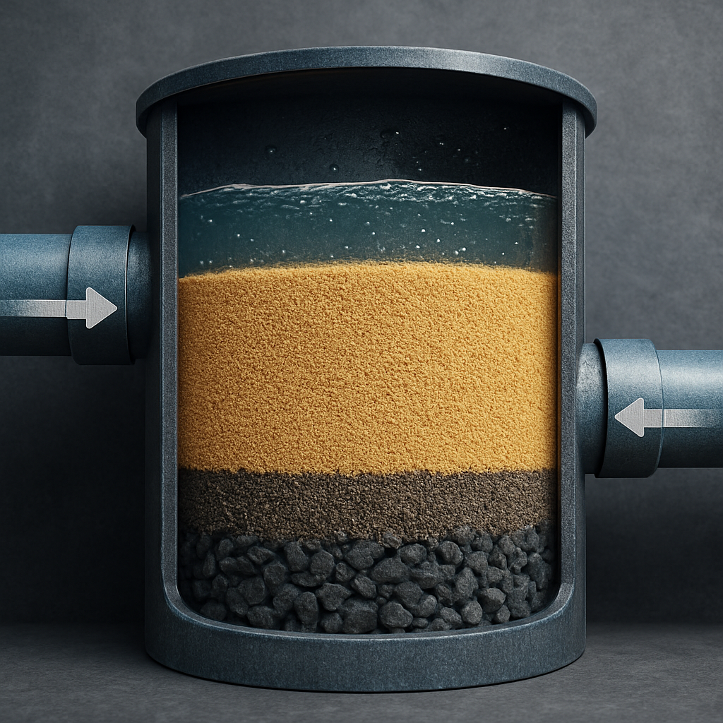
3. Media Selection and Bed Configuration
Media choice drives both particle capture and operating profile. The two numbers you must require on purchase and verify on delivery are d10 (effective size) and Cu (uniformity coefficient) – everything else flows from those metrics. Specify acceptable ranges in the contract, insist on sieve certificates, and require a small-sample bench test that reproduces your planned backwash sequence.
| Media | Typical d10 (mm) | Typical Cu | Practical note |
|---|---|---|---|
| Anthracite | 0.9 – 1.7 | 1.6 – 2.5 | Top layer – coarse and low density to capture larger particles and extend run length |
| Silica sand | 0.45 – 0.55 | 1.3 – 1.8 | Middle layer – primary mechanical filtration, choose washed, low-fines sand |
| Garnet/Heavy mineral | 0.2 – 0.4 | 1.4 – 2.0 | Bottom layer – high density, fines capture and stable support above underdrain |
Layer depths are a function of solids load, desired run length, and backwash capacity. Typical multimedia beds use a deeper top layer and progressively thinner dense layers below. Deeper beds improve capture and damp transient spikes, but they increase clean-bed headloss, backwash volume, and media attrition risk. Specify depth ranges in both SI and US units and tie the buyer warranty to attrition limits after a defined number of backwash cycles.
Field verification and acceptance
- Require sieve analysis: Provide
d10,d50,d60and calculateCuon delivery samples. - Attrition test: Contract a mass-loss test after 50 simulated backwashes or a vendor-provided accelerated abrasion report.
- Backwash expansion test: Measure percent expansion at design air-water scour rates during commissioning and verify no media carryover.
- Visual and mass balance check: After initial wash, confirm fines downstream are within project limits and record percent mass retained.
Concrete example: A municipal tertiary reuse project swapped single-media sand for a three-layer anthracite-sand-garnet bed after pilot trials showed frequent early breakthrough. The multimedia bed doubled practical run length under variable upstream loads, but required a 15 to 20 percent increase in backwash volume and a specification change to require vendor attrition < 2 percent per 1,000 cycles.
Judgment that matters: Many teams pick media by price and assume sieved sand is homogeneous. That is a false economy. Cheap sand with high fines will shorten runs, triple backwash solids, and force premature media replacement. When footprint is constrained, invest in graded multimedia and a proven underdrain – you buy operational stability, not just initial area savings.
d10 and Cu thresholds, require attrition and expansion tests in the purchase spec, and tie acceptance to measured backwash carryover. For contract language examples and lab test protocols see Filter Media Selection and Testing and AWWA M37 at AWWA M37 Filtration Manual.4. Hydraulic Design: Underdrains, Distribution, and Flow Uniformity
Hydraulics at the media-bottom interface decide whether a sand filter performs or fails. A well-selected underdrain with verified distribution removes guesswork; a poor one creates channeling, localized media scour, and unexplained turbidity spikes that operators fight for years.
Pick underdrain type against realistic maintenance and solids conditions, not vendor brochures. Molded multiport systems give the best protection against media migration and tolerate higher air-scour rates, but cost more up-front and are harder to inspect in-situ. Lateral-collector systems are easy to repair and cheap, yet they clog or leak preferentially if influent solids are poorly controlled. Radial or hub-and-spoke assemblies strike a balance when space for access is planned.
Practical check: size laterals so that individual lateral flow at peak design does not exceed the value the manufacturer rates for solids transport; verify lateral headloss is less than a modest fraction of your clean-bed headloss so the underdrain does not dominate differential head signals used for run termination. When in doubt, require vendor hydraulic curves in the spec and insist on a factory-witnessed flow test.
Commissioning and diagnostic tests
- Air/water distribution test: Run air-only then air+water at design scour rates and verify visually and with pressure taps that no lateral is starved; acceptance target: flow variance across laterals within ±15%.
- Tracer/short-circuit test: Inject a conservative dye or conductivity slug at the inlet headers and measure breakthrough times at each lateral row to detect hydraulic dead zones or preferential paths.
- Differential head mapping: Map clean-bed differential head across the bed and repeat at incremental filtrate flows; large local deviations indicate underdrain blockage or cracked laterals.
- Media expansion verification: During air scour, verify top-layer expansion is uniform and no fines pass the underdrain; set carryover limits in the specification and record turbidity of washwater.
Trade-off that matters: maximizing air scour intensity shortens run recovery time but increases risk of localized media movement and underdrain abrasion. Design your air-scour to achieve 20-30% bed expansion in tests rather than to an arbitrary high flow—most gains occur early and the extra stress beyond that causes attrition without better cleaning.
Concrete example: In a municipal tertiary filter retrofit, operators replaced failing PVC laterals with a molded multiport underdrain and reconfigured inlet distribution plates. Instant result: media loss stopped and run length increased from about 14 hours to 60 hours under the same influent load. The retrofit required changing the backwash sequencing (lower instantaneous air but longer, gentler water rinse) to protect the new media and underdrain.
Common oversight: designers often treat inlet weirs and distribution troughs as trivial. Uneven inlet velocities and high local approach velocities cause surface channeling and premature turbidity breakthrough. Keep inlet velocities low, provide baffling or perforated distribution boxes, and hydraulically model the inlet when filter aspect ratio is extreme.
Next consideration: after underdrain and inlet work, tie your differential head alarms and effluent turbidimeter to the verified hydraulic baseline. If your baseline is wrong you will chase symptoms rather than fix the hydraulic root cause.
5. Backwash and Air-Scour Design and Waste Management
Direct point: Backwash is not a hygiene ritual — it is the operational lever that determines run length, media life, and solids disposal costs. Design the sequence and waste path to control peak flows, protect the underdrain, and keep suspended solids from returning to the headworks where they eat clarifier capacity.
Sizing logic and pump capacity
How to size instantaneous backwash flow: compute Qbw = Abackwashed × vbw, where Abackwashed is the total planimetric area of filters you will wash at once and vbw is the chosen wash intensity (expressed as m3/m2·h or equivalent). For pump selection, convert Qbw to m3/s, add a safety margin (15 to 25 percent) and design head as the sum of static lift, friction through pipes and valves, and allowance for surge. Do the same for air blowers: match blower capacity to the underdrain manufacturer curve at the selected scour pressure.
Practical judgement: do not design to wash all filters simultaneously unless you have proven headworks/clarifier capacity and discharge consent. It is usually better to size plumbing for two or three concurrent cells and accept a larger number of smaller pumps or variable-frequency drives to reduce peak power and allow staged recycle.
Sequence design and control targets
- Step 1 — short air pulse: brief high-velocity air-only pulse to mobilize trapped solids at the media surface and break surface seals. Use a controlled burst rather than continuous high-pressure air to avoid fluidizing the whole bed.
- Step 2 — combined air+water scour: follow with simultaneous air and water to expand the bed and shear interstitial solids; monitor for carryover at the underdrain sampling point and reduce air if fines pass.
- Step 3 — water rinse: finish with water-only flushing until effluent turbidity from the backwash line drops below your reuse/discharge threshold or until clarifier feed meets solids concentration targets.
Control logic: combine differential-head and effluent turbidimeter signals to end the rinse. In practice, end-rinse triggers tied to a descending turbidity trend and a minimum elapsed rinse time prevent premature termination that leaves fines behind.
Trade-off to own: stronger, longer scours improve cleaning but accelerate media attrition and increase fines generation. If you see diminishing returns in headloss recovery after increasing scour intensity, you are wearing the media more than cleaning it — back off and increase backwash frequency instead of amplitude.
Waste handling options and selection criteria
Options: direct discharge, recycle to headworks, recycle to a dedicated backwash tank with clarification, or pumped to a sludge handling train. Choose based on solids concentration, regulatory discharge limits, and capacity of upstream processes.
Key limitation: recycling backwash to headworks without pre-thickening or a buffer often overloads the clarifier and degrades solids removal efficiency. If you must recycle, provide a buffer tank sized to smooth cycles and a means to remove concentrated solids to prevent return-to-influent spikes.
Concrete example: A 5,000 m3/day tertiary plant moved from direct discharge to a two-stage approach: backwash went to a 100 m3 buffer tank with quiescent settling, then the clarified overflow returned to the headworks and the settled solids were pumped to a sludge thickener. After the change, operators halved peak TSS loads to the clarifier and reduced the number of emergency clarifier bypass events during wet weather.
Operational insight: invest in a modest buffer and a simple solids removal step — it costs less than repeated clarifier upgrades and prevents the common cycle of backwash recycle creating the very spikes you designed the filters to remove.
Final consideration: design backwash hydraulics and the waste path together. If you treat them as separate problems you will undersize one or the other and pay in lost runs, media replacement, or downstream headaches. For commissioning checks, run a full-scale backwash acceptance test with turbidity and solids sampling and verify that your control logic and buffer sizing keep clarified return concentrations within agreed limits.
6. Instrumentation, Monitoring, and Run Optimization
Instrumentation and placement decide whether your control strategy is actionable or just noise. Pick sensors for reliability in a dirty, wet environment and place them where the signal relates directly to the filter process rather than where it is convenient for wiring.
Minimum instrument set. Install influent and effluent turbidity sensors with flow-through cells and automatic wipers, differential-head transducers monitoring the filter bed, a flow meter per filter or per filter bank, and temperature/pH where chemistry affects coagulant behavior. Consider an online particle counter or UVT sensor where organic/colloidal matter drives breakthrough risk.
Siting and maintenance details that matter. Mount turbidity probes in stilling wells or sample chambers sized to eliminate bubbles and entrained air; do not place probes in free-surface troughs unless you add degassing. Use a bypass sample loop with a constant sample flow and a quick-connect port for grab-sample validation. Specify automatic wipers, scheduled zero checks, and a documented calibration frequency tied to raw-water variability — sensors left to drift cause unnecessary backwashes and operator override culture.
Control logic — combine level and trend, not single events. Use a two-tier approach: advisory alarms on short turbidity spikes or small headloss changes, and trip logic for sustained excursions. Practical rule: trigger operator review when effluent turbidity rises above 0.25 NTU for a rolling 10-minute window or when differential head rises faster than 0.01 m H2O per hour; only auto-initiate backwash on a sustained signal or combined turbidity + headloss trigger to avoid false cycles from transient upstream events.
Data workflows for tuning and run optimization. Record raw high-frequency signals and a downsampled engineering dataset for trend analysis. Monitor moving-average turbidity, derivative of differential head, and event tags (coagulant dose changes, tank cleaning). Use these to derive simple heuristics: dynamic backwash scheduling based on combined metrics, staged backwash of a subset of filters, and automatic hold-off timers after chemical feed changes. Machine learning can find non-obvious correlations, but in practice it only pays off if you have months of clean, labeled historical data and an engineer to validate the model.
Practical trade-off and common mistake. Investing in expensive sensors before fixing hydraulics is backward. Good instrumentation amplifies a well-built process; it does not compensate for poor underdrain distribution, uneven inlet weirs, or media grading problems. Expect a short period of tuning after commissioning where operator judgment sets false-positive tolerances.
Concrete example: A municipal tertiary plant replaced fixed-interval backwash with a combined turbidity+differential-head strategy and instrument upgrades. After three months of tuning the thresholds and adding a short validation delay, average backwash frequency dropped from daily to roughly once every 2.2 days and backwash volume fell by about 28 percent; coagulant usage also decreased because dosing responded to real-time turbidity trends rather than fixed setpoints.
7. Troubleshooting Common Performance Problems
Direct statement: Most recurring sand filtration failures are hydraulic or media-related, not mysterious chemistry problems. Diagnose with a short, prioritized checklist and measure before you escalate operational intensity — heavy-handed fixes (more air, longer scours, higher dosing) usually trade a short-term gain for faster media attrition and higher solids in the backwash stream.
Symptom-driven diagnostic workflow
Start small, act fast. When a symptom appears (short runs, turbidity breakthrough, media loss, or high irreversible headloss), follow a consistent workflow: contain the problem, collect targeted measurements, run quick field tests that isolate hydraulics from chemistry, then apply the least invasive corrective action that addresses the root cause.
- Contain: put the affected filter on
filter-to-wasteor divert effluent until you understand whether the failure is solids carryover or true filtrate quality loss. - Measure: record influent/effluent turbidity, differential head trend, raw-water particle-size snapshot, and backwash turbidity/SS during the next wash.
- Isolate hydraulics: run a brief underdrain air/water distribution check and a tracer slug to detect channeling before changing chemical regimes.
- Act conservatively: adjust coagulant only if jar tests support it; otherwise prefer controlled backwash sequence changes and targeted underdrain repairs.
Field tests that tell you what broke
Practical field tests and what they reveal. These are cheap, fast, and diagnostic — do them in this order to avoid unnecessary interventions.
- Underdrain air distribution test: run incremental blower steps and verify equal lift or pressure across zones; non-uniformity points to blocked laterals or cracked manifolds.
- Tracer slug (conductivity/dye): a fast breakthrough at the effluent indicates surface channeling or inlet short-circuiting rather than media failure.
- Media grab and sieve: a few scoops near suspected zones will reveal fines migration, compaction, or lost grading — compare to the purchase
d10/Cucertificate. - Backwash-rinse sampling: measure SS and turbidity at 1-minute intervals during rinse; prolonged elevated values after a correct rinse point to internal fines (attrition) or broken underdrain elements.
Judgment call that matters: if hydraulic tests show distribution problems, stop changing chemical dosing. Fix the hydraulics first; better chemistry cannot hide channeling or starved laterals and will only increase sludge load downstream.
Prioritized remedial actions
- Immediate containment (minutes): place filter on waste, reduce surface loading on adjacent filters, and notify operations with a clear action plan.
- Short-term fixes (hours): intensify backwash within manufacturer limits (longer rinse, add a gentle combined air+water step), but do not exceed the underdrain's rated scour pressure or media expansion — that accelerates wear.
- Medium-term repairs (days-weeks): repair or replace blocked laterals, rebalance inlet distribution, and replace top 10-20% of media if lab sieve shows significant fines.
- Long-term changes (weeks-months): redesign underdrain or inlet headers if tracer and distribution tests repeatedly fail, or move to graded multimedia if single-media beds cannot meet variability without excessive backwash.
Trade-off to accept: aggressive short-term cleaning recovers effluent fast but increases the chance you will need full media replacement sooner. Sometimes spreading smaller, more frequent backwashes with gentler air instead of a single heavy scour preserves media life and lowers lifetime cost.
Concrete example: A wastewater reuse plant experienced run length contraction from 96 hours to about 12 hours after storm-season loads jumped and headloss rise accelerated to about 0.9 in H2O per hour. Operators first put the filters to waste, ran a targeted underdrain air distribution test (which showed two starved lateral zones), then performed a controlled backwash sequence on the affected cells and repaired clogged laterals the next day. Full run length recovery took four days while upstream coagulation was retuned to the new seasonal particle-size distribution.
Emergency action: if effluent turbidity remains high after containment and a proper wash, hold the filter out of service and route all flow through validated filters or polishing — do not let suspect filtrate reach downstream reuse or drinking-water points.
Final takeaway: build a concise troubleshooting playbook into your O&M manual that pairs symptoms with the specific measurements above and a prioritized set of fixes. That discipline prevents knee-jerk escalation, protects media life, and focuses capital where it actually reduces recurrence.
8. Design Checklist, Sample Specification Table, and Commissioning Protocol
Start here: lock the procurement and acceptance language before you pick a contractor. Most filter failures trace back to vague specs that allow substandard media, underdrains, or insufficient factory testing — fixable only with retrofit expense and downtime.
Design and procurement checklist
Media verification: require signed sieve certificates with d10 and Cu, supplier attrition data, and a small-sample bench backwash/expansion test witnessed by your engineer or an independent lab. Do not accept bulk delivery without this evidence.
Underdrain performance: demand vendor hydraulic curves, rated air scour capacity, and factory witness of a flow distribution test. Put a hold point in the contract that permits site verification before final payment.
Backwash capacity and sequence: specify the peak backwash flow you will permit to run concurrently and require pump/blower curves sized to that duty with a margin. Specify control logic blocks for air-only, combined air+water, and rinse steps in the PLC narrative.
Instrumentation and data requirements: list required sensors, sample-cell arrangements, auto-wipers, calibration intervals, and SCADA data tags for turbidity (influent/effluent) and differential head. Require spare probes and documented maintenance procedures in the O&M manual.
Acceptance testing scope: include hydraulic distribution checks, media expansion/carryover limits, seeded challenge or equivalent proof-of-performance, and a stability observation period under actual plant loading.
Sample specification snapshot (contract-oriented)
| Specification Item | Requirement (worded for contract) | Acceptance method / Pass criteria |
|---|---|---|
| Media grading and attrition | Supplier to provide sieve analysis (d10, d50, d60), attrition report, and 20 kg demo sample for bench testing | Bench backwash reproduces no visible carryover and lab sieve within 10% of certificate |
| Underdrain hydraulic performance | Provide manufacturer curve and guaranteed distribution uniformity; rated air scour at working pressure | On-site air/water distribution test: uniformity confirmed against manufacturer curve and no starved zones |
| Backwash pumps and blowers | Deliver pumps/blowers with verified duty at design simultaneous-wash condition plus 20% mechanical margin | Factory curve review and on-site performance run at design head |
| Instrumentation | Influent and effluent turbidity, differential head transducers, flow meters per filter bank, with maintenance spares | Probe calibration checks and trending validation during commissioning |
| Performance run | Manufacturer to demonstrate stable operation under normal plant loading for an agreed observation window | Seeded-challenge or equivalent showing filtrate quality meets owner target for the window; documentation required |
Commissioning protocol (condensed and actionable)
Phase 1 — dry checks and factory witness: confirm as-built underdrain geometry, pipework, valves, and electrical terminations. Witness vendor factory tests or review video evidence for critical items if factory attendance is impossible.
Phase 2 — hydraulic baseline: fill and run each cell at minimum and design filtrate flows; map differential head across zones and record clean-bed head. Establish these records as the SCADA baseline.
Phase 3 — distribution and expansion verification: perform staged air and air+water tests while sampling underdrain discharge for carryover. Adjust blower setpoints to reach the vendor-specified expansion without fines passing the underdrain.
Phase 4 — performance proof and tuning: run at projected loading for the observation window. Execute at least one seeded-challenge or worst-case influent simulation, verify effluent turbidity behavior, tune backwash timing and PLC logic, then run a stability window under normal operation.
Phase 5 — handover and documentation: deliver calibrated instruments, O&M manual with step-by-step backwash recipes, spare parts list, and a 90-day tuning support period where vendor support includes adjustments after real raw-water variability is observed.
Do the distribution and expansion tests before the seeded challenge. If hydraulics are off, any performance test is misleading.
Concrete example: a reclaimed-water project added the procurement hold points above after a prior retrofit failed. The new vendor performed a witnessed bench expansion and on-site distribution test; the owner caught a lateral-pack sizing error before filling media, avoiding a lengthy and costly underdrain replacement.
Next consideration: if you cannot secure contract hold points or factory witnesses, allocate contingency budget and schedule for an early-season field inspection and a possible underdrain retrofit — plan for it up front rather than discover it under load.